AaronTools and Matplotlib

You can download the Jupyter Notebook version of this page here (click “Download raw file”).

AaronTools Geometry objects can be plotted within Matplotlib figures using ‘HoukMol’ style (you’ll recognize it when you see it).

For instance, if we just want to generate a HoukMol style image of a molecule, we can create an empty Matplotlib figure/axis, set a reasonable scale, set the aspect to ‘equal’ and then plot the molecule:

from AaronTools.geometry import Geometry
import matplotlib.pyplot as plt

# Create AaronTools geometry
geom = Geometry.from_string('toluene', form='iupac')

fig, ax = plt.subplots() # create figure and axis
ax.axis('off')           # hide axes
ax.set_xlim(-5,5)        # set scale for x-axis
ax.set_aspect('equal')   # set aspect to 'equal'
geom.plot(ax, fig)       # plot molecule
plt.show()

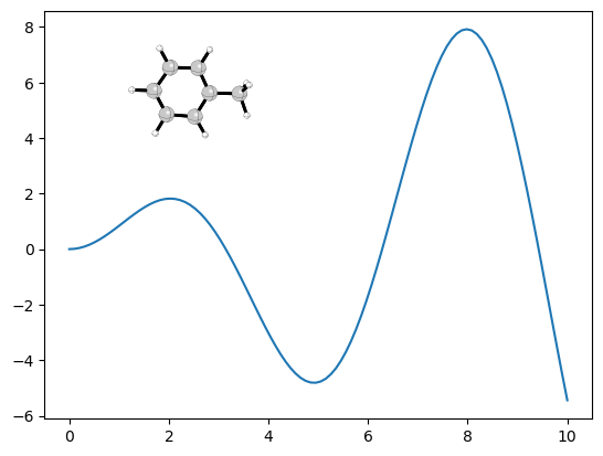
If we want to insert a molecular structure into a plot of data, we need to create a subplot in order to control the scale of the molecular structure.

We will also need to set both the x- and y-limits to enable control over the vertical and horizontal placement of the molecule within the plot.

from AaronTools.geometry import Geometry
import matplotlib.pyplot as plt
import numpy as np

# Create dummy plot of data as an example
x = np.linspace(0, 10, 100)
fig, ax = plt.subplots()
plt.plot(x, x*np.sin(x))

# add subplot to hold molecular structure figure
ax2=fig.add_subplot(111, label="HoukMol", frame_on=False)
ax2.axis('off')
ax2.set_xlim(-10, 10)
ax2.set_ylim(-10, 10)
ax2.set_aspect('equal')

# Create AaronTools geometry
geom = Geometry.from_string('toluene', form='iupac')
# Shift geometry to place it within overall figure
geom.coord_shift([-6, 6, 0])
# Plot AaronTools geometry
geom.plot(ax2, fig)
plt.show()

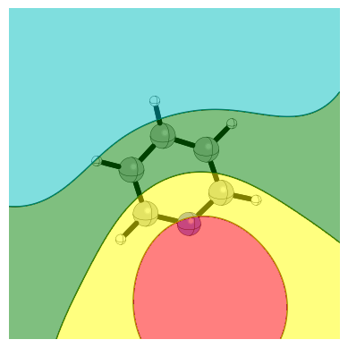
Finally, one of the most useful aspects of being able to plot AaronTools geometries within a Matplotlib figure is to superimpose computed molecular data over top of a HoukMol style molecule.

For example, below we use Psi4 to calculate the electrostatic potential (ESP) in the plane 3.5 A from pyridine at the HF/STO-3G level and then make a semi-transparent contour plot of this data on top of a HoukMol figure of pyridine at the same scale.

In this way, we can visualize the ESP (or other data computed on a grid) in the vicinity of a molecule!

from AaronTools.geometry import Geometry
import psi4
import psi4.core as p4c

# Build Geometry and convert to Psi4 molecule object
geom = Geometry.from_string('pyridine', form='iupac') # Will be *close* to being in the XY plane
mol = geom.convert_to_Psi4()

# build grid to compute ESP on
xgrid = np.linspace(-5, 5, 100)
ygrid = np.linspace(-5, 5, 100)

# build 2D meshgrid
x, y = np.meshgrid(xgrid, ygrid)

# Get HF/STO-3G wavefunction using Psi4
psi4.set_output_file("output.dat", False)
energy, wfn = psi4.energy('scf/sto-3g', return_wfn = True)

# Build 3D grid in z = 3.5 A plane and setup ESP calculation on grid
points = np.vstack([x.ravel(), y.ravel()] + [np.array([3.5]*xgrid.size*ygrid.size)]).T
psi4_matrix = p4c.Matrix.from_array(points)
myepc = p4c.ESPPropCalc(wfn)
psi4.set_num_threads(8, quiet = True)

# Calculate ESP and convert to kcal/mol
ESP = 627.51*np.array(myepc.compute_esp_over_grid_in_memory(psi4_matrix))

# Convert ESP to 2D array
ESP = ESP.reshape(x.shape)

# Make contour plot superimposed over HoukMol image
ESPmax = 5
ESPmin = -5
scale=np.arange(ESPmin, ESPmax, (ESPmax - ESPmin)/5)

fig, ax = plt.subplots()
ax.set_aspect('equal')
ax.axis('off')

CS = ax.contour(x, y, ESP, scale, colors='k',linewidths=1, zorder=10, linestyles='solid')
CSF = ax.contourf(x, y, ESP, scale, colors=('r','yellow','g','c','b'), alpha=0.5, extend='both', zorder=10)
geom.plot(ax, fig)
plt.show()